If CAP were real-time: adding timing requirements to the definition of availability

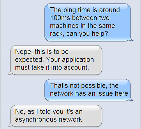
“If you are not too long, I will wait here for you all my socketReadTimeout.” - Oscar Wilde, quoted from memory.

This post is part of the CAP theorem series. You may want to start by my post on ACID vs. CAP if you have a database background but have never really been exposed to the CAP theorem. The post discussing some traps in the ‘Availability’ and ‘Consistency’ definition of CAP could also be used as an introduction if you know CAP but haven’t looked at its formal definition.

Delays are a hot source of confusion when using CAP. Confusion arises out of the understanding of what an asynchronous network--the network model used in the CAP proof--actually is. Confusion arises out of what TCP is exactly. Confusion arises out of the definition of availability in CAP--which does not have any timing requirement.

In this post, I’m not only going to cover why speaking about delays when the network is asynchronous is a mistake or why TCP is more than an asynchronous network: I will also show that adding timing requirements to CAP makes it usable not only for partitions but also for delays.

Why are there never any delays in academic networks?

The CAP proof by Gilbert and Lynch uses an “asynchronous model, in which system components take steps at arbitrary speeds.” The key point is that there can be no delay, because there is absolutely no timing guarantee, so a message is never late. That’s by design, as stated by Lynch: “algorithms designed for the asynchronous model are general and portable, in that they are guaranteed to run correctly in networks with arbitrary timing behavior.”

On such a network model, you cannot build an application that needs a guaranteed response time. You cannot even provide an approximation of its expected response time. You can at best prove that the application will answer… someday. You can calculate the number of messages required by a given protocol, but you cannot, in any case, calculate a response time.

Such a network is never sufficient to write a real-life application: a real-life application must provide its results within a reasonable timeframe. It so happens that you can build real-life applications on top of TCP for a simple reason: TCP is asynchronous, yes, but it is not only asynchronous.

TCP or You Have a Clue About the Actual Communication Time

TCP: you don’t want to have this conversation.

TCP is not an easy protocol. The congestion avoidance algorithm has changed many times. Some gateways trick the congestion avoidance algorithm to “regulate” applications. And there are many different options, with some of them conflicting between themselves. Modeling a TCP network is incredibly difficult, and is worthy of a PhD. It creates value, however. For example, there are works about improving the model to increase router capacity: “Current backbone routers typically contain extremely large buffers. [] this rule of thumb overprovisions buffers by several orders of magnitude [] the TCP flows can be modeled as independent, and therefore, by the law of large numbers, the total number of TCP packets in the network converges to a Gaussian distribution.”

This is complex, and most of us don’t have a PhD in TCP modelization.

However, we all have in our minds a simplistic model of how TCP works: if we’re in a LAN, we expect a roundtrip to take a few milliseconds at most. On a WAN it can go up to 200 milliseconds. And we expect some correlation: if a roundtrip needs 10 seconds, then the next roundtrips are likely to need 10 seconds as well. This is a model, and it does take time into account. It uses a fixed round-trip time, so it does not capture most of the TCP richness, but it’s the one commonly used for back-of-the-envelope calculations.

The model to choose depends on what you want to achieve. In any case, if you want to speak about response time, you need a network model that includes time.

Real-time availability

CAP definition of availability is quite clear: “For a distributed system to be continuously available, every request received by a non-failing node in the system must result in a response.” There is no mention of time, which is logical with a pure asynchronous network.

Many web applications do care about time however. They do have a time limit: after a given amount of time, the user will stop waiting for an answer and will move on to another web-site. That’s exactly what a real-time time system is. Then what Shin & al. wrote is an exact match for us: “It is often assumed that the availability and reliability requirements of a system can be addressed independent of its timing constraints. This assumption, however, does not consider the distinguishing characteristic of real-time computing: the correctness of a system is dependent not only on the correctness of its result, but also on meeting stringent timing requirements.”

In a hard real-time system, “not in time” is equivalent to “failed”. For example, if you take a photo of an athlete crossing the finish line, taking it one second too late is equivalent to not taking it at all. Many applications are soft real-time: if the operation is done after the time limit the value decreases but it’s not zero. In both cases a common practise is to measure the number of operations that were beyond the time limit. This gives for example, “the system should perform an activity before time t in 92% of the cases” (even if it’s not perfect for a soft real-time system, as you need to look at all percentiles, it’s simple and enough for most cases). One could say that most systems are actually real-time: “Non Real-Time Systems [exist], however in most cases the (soft) real-time aspect may be constructed (e.g. acceptable response time to user input).” In any case, real-time is not about being fast, interactive or reactive: it’s just about meeting timing requirements.

So what about adding some real-time in CAP? Let’s change our definition of availability to include it. It gives (in bold what I have added to the proof’s definition): “For a distributed system to be continuously available, every request received by a non-failing node in the system must result in a response within a given deadline.”

This small change leads to an ocean of questions, and CAP will help us answer at least one of them. Let’s look at a simple system:

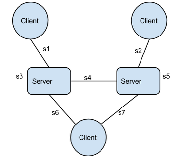
We have 7 latency sources, numbered s1 to s7:

• the links themselves
• the operation time (s3 & s5), that can vary for many reasons, such as garbage collections.

Which ones--if any!--of these latency sources, alone or combined, will force us to choose between real-time-Availability and Consistency?

Here CAP helps us answer s4, the link between the two servers. When s4 is greater than twice the required response time we cannot be available and consistent. The two servers may each need to answer multiple requests without being able to communicate between themselves: they are effectively partitioned during this timeframe, so CAP applies and we have to choose between consistency and availability.

This proves that you have to choose between availability and consistency in at least one case.

What about the other latency sources?

It’s also possible to prove that in some cases forfeiting consistency will improve the  real-time-availability. Using the deployment presented on the schema above, let’s imagine a distributed system with an asynchronous replication between the two servers. The client sends its queries to the two servers and waits until one of them answers. This system is obviously not consistent, but the response time will be great:

min ( s6+s3, s7+s5 )

It’s not possible to beat this: any other distributed system, consistent or not, will include more latency sources. For example, the client can send a message to both servers and wait for both of them to answer. This gives:

max ( s6+s3, s7+s5 )

Or the servers can communicate between themselve. This will give something like:

s6 + max ( s3, s4+s5 )

or

s6 + s3 + s4 + s5

There are many possible variations. But all of them will include more latency sources than our first version.  In other words, for some deadlines and some operations a consistent system is less available than the non-consistent system: CAP strikes again: you have to choose between availability and consistency.

Applied to real-life systems, it means that it’s possible to build an eventually consistent system that will have a better availability than any consistent one when facing delays caused by GC or erratic i/o. This formalizes what people have been saying about GCs and delays: there is a trade-off between availability and consistency. It’s wrong when applied to the standard CAP, but it becomes true with the real-time CAP.

How much more available?

Can we have a hint of how much availability we have to trade for strong consistency? Let’s try.

The math

Let’s consider that all latency sources can be modelized by a Gaussian and are independent.

We can have this:

	average (ms)	standard deviation
network client to server (s1, s2, s6, s7)	100	5
operation time (s3, s5)	10	1
network between the servers (s4)	1	1
Response time deadline	150

The results are, as you can guess:

Availability Eventually Consistent	100%
Availability Strongly Consistent (any implementation)	100%

In other words, they are both available, in this case because the s4 value is quite small compared to the required response time. That’s often the case with a web-site: if the objective is to read a value from memory to return it to a client behind a WAN, there is not real question on the pure delay side: the WAN dominates everything.  There are many variations around this, for example if s7 is very high.

But let’s look at a more interesting example. If we consider that the client is closer to the server on a reliable network, but with less reliable servers:

	mean (ms)	standard deviation
network client to server	2	0
operation time	15	3
network between the servers	2	0
Response time deadline	20

Here we have:

Eventually Consistent min(s6+s3, s7+s5)	97%
Strongly Consistent s6+s3+s4+s5	0%
Strongly Consistent max(s6+s3, s7+s5)	70%
Availability Strongly Consistent s6+max(s3, s4+s5)	53%

Here the differences become visible. Let’s look at them:

• 97% vs. 0%: the mean time of s6+s3+s4+s5 is 34. The target being 20, it’s just impossible. We add a sequential and synchronous call to the first call, and it has a cost. Strong consistency is more expensive than eventual consistency, so by choosing the target value accordingly, we can have whatever gap we want: a target of 20ms if the sum of the mean time is 34ms is not really reasonable.
• 97% vs. 70%: That’s the difference between waiting for a single answer or from an answer from all servers. The more variance the higher the difference here. That’s the real choice between availability and consistency.
• 53% vs. 70%. That’s the cost of the two extra 2ms added by the communication between the servers.

We’re seeing here that the consistency cost can be split in 2 different categories. Either there are more steps (i.e. this increases directly the mean time), either there are less hedging/speculative execution options (i.e. this increases the sensitivity to variance).

The First Limit of the Exercise--Durability Comes at a Cost

In the calculations above, there is a huge difference because the strongly consistent system has to wait from an answer from the two servers, while the eventually consistent one only needs a single server to answer. That’s simple. But something often forgotten when looking at distributed databases with the CAP point of view is durability: people do synchronous writes not only for consistency but also for durability. Traditional SQL databases replicate on multiple disks. Most of the NoSQL generation replicate on multiple nodes. In both cases the durability comes from the synchronicity.

In other words, being less sensitive to erratic delays is a good reason to do only asynchronous communications between the servers, but durability is a good reason to do exactly the opposite, especially for NoSQL databases deployed on commodity servers.

The Second Limit of the Exercise--Modelization is Difficult

The calculations above were done with some assumptions:

• It presupposes a Gaussian model to be a good fit. Is it true for a network on a LAN? For an application that can have GC, i/o, queuing effects between queries? Maybe locks between queries?
• It presupposes independence between the different latency sources. That makes things simpler. It may not be realistic however. Herd effect is a well known counter-example.
• It assumes a simplistic database implementation. The database can be written in many different ways. As we see when we compare “max(s6+s3, s7+s5)” to “s6+s3+s4+s5” it has a real impact. So the DB implementation must be modelized accordingly.
• It presupposes a single kind of operation: all the operations go to the two servers. But a dynamo-like system with N=2 W=2 and R=1 will not replicate the reads. If the workload is dominated by reads, the consistent system will be as available as the non consistent one. This means the application must be modelized as well to understand the trade-offs.

In other words, this post does not solve the debate over consistency models. Some design decisions are not driven by CAP and quantifying the result is very difficult. This is not new, and to quote Shin again: “Determining the timing constraints on a system from its availability requirements is a very difficult problem.”

Are the delays coming from latency sources the same as partitions?

No. There are delays. Making the distinction is important: most real-life systems manage differently partitions and delays. For example, let’s look at HDFS (Hadoop Distributed File System):

What	timerange	Decision
Request takes longer than usual or than specified.	milliseconds	Hedge reads: start a parallel call on another node. (HDFS-5776)
No heartbeat for a while, but not yet a timeout.	seconds	Stale node: avoid this node whenever possible (HDFS-3703)
Heartbeat timeout.	minutes	Partition: considers the nodes and their data as lost, replicates again from the accessible nodes for safety.

Partition and delay are different things and they will be managed differently in practice.

Latency & real-time

The trade-off between consistency and latency was already detailed by Daniel Abadi: PACELC is about splitting the problem in two parts:

• PAC in PACELC is for the choice between consistency and availability when there is a partition
• ELC in PACELC is for the choice between consistency and latency when the system is not partitioned.

Adding timing requirements to the definition of availability is quite natural however. Saying “+100 ms => -1% sales” is saying “my web-site is a soft real-time system.” It’s also very intuitive and this explains, in my opinion, why so many people use CAP when reasoning about delays.

Conclusion

The asynchronous model is there to get time questions out of the way: speaking about delays with this asynchronous model is meaningless. However, we can take time into account in a TCP model--and we all do it to write real-life applications. Moreover, by including the time in the definition of availability used by CAP, we find a consistency vs. availability trade-off.

Defining good models to quantify this trade-off is another question, and a far more complex one. The design is also constrained by other requirements beyond consistency alone: durability imposes synchronous writes whatever the consistency model.

	This post is part of the CAP theorem series
⇐ CAP applied: Optimizing for process crash		CA again ⇒